

Why Estimates Below the Minimum Detectable Effect Can Be Statistically Significant


When designing a study to estimate an effect—such as that of a treatment, service, or public program—researchers often calculate the effect size that is likely to result in a statistically significant finding. This size is called the study’s minimum detectable effect. If the minimum detectable effect is too large, the study is unlikely to produce a statistically significant estimate even if the program is effective, so researchers may increase the sample to reduce the minimum detectable effect. This blog post addresses a common misconception about minimum effect sizes: that estimates smaller than the minimum detectable effect cannot be statistically significant. In fact, estimates smaller than the minimum detectable effect can be and often are statistically significant. This post explains why, and what that fact means for interpreting study results.
Which Estimates Are Statistically Significant
If researchers conducted 100 studies, they would get 100 different effect estimates even if the true effect were the same across studies, because a single study’s estimate reflects not only the effect but also the sampling error from the study’s sample. (Box 1 explains the true effect and an estimated effect.)
Box 1. True Versus Estimated Effects
True effect: The actual effect of an intervention. The actual effect cannot be directly observed.
Estimated effect: The effect computed from data in a study. The estimate will depend on the sample that is included in the study.
Figure 1 illustrates this point. The blue bell curve is centered at 0 and represents the distribution of estimates if the true effect were 0. Estimates close to 0 are more likely than estimates further from 0. The distribution is bell-shaped because as the sample size gets larger, the effect estimates follow Student’s t-distribution and eventually follow a normal distribution, both of which have a bell shape.[1] The distribution’s width is determined by the study’s standard error, with larger samples and more balanced designs (that is, designs with comparably sized treatment and comparison groups) producing smaller standard errors and thus narrower distributions.[2] The figure contains a vertical black line at a value of 1.96 standard errors above zero. This value is important for the following reason: An estimated effect is different from 0 to a statistically significant degree at the 5 percent significance level if it is more than 1.96 standard errors larger or smaller than 0.[3] Any estimate to the right of that line will be statistically significant while estimates to the left of that line will not be.
Figure 1. Minimum Detectable Effect Versus
Statistically Significant Effect Estimates
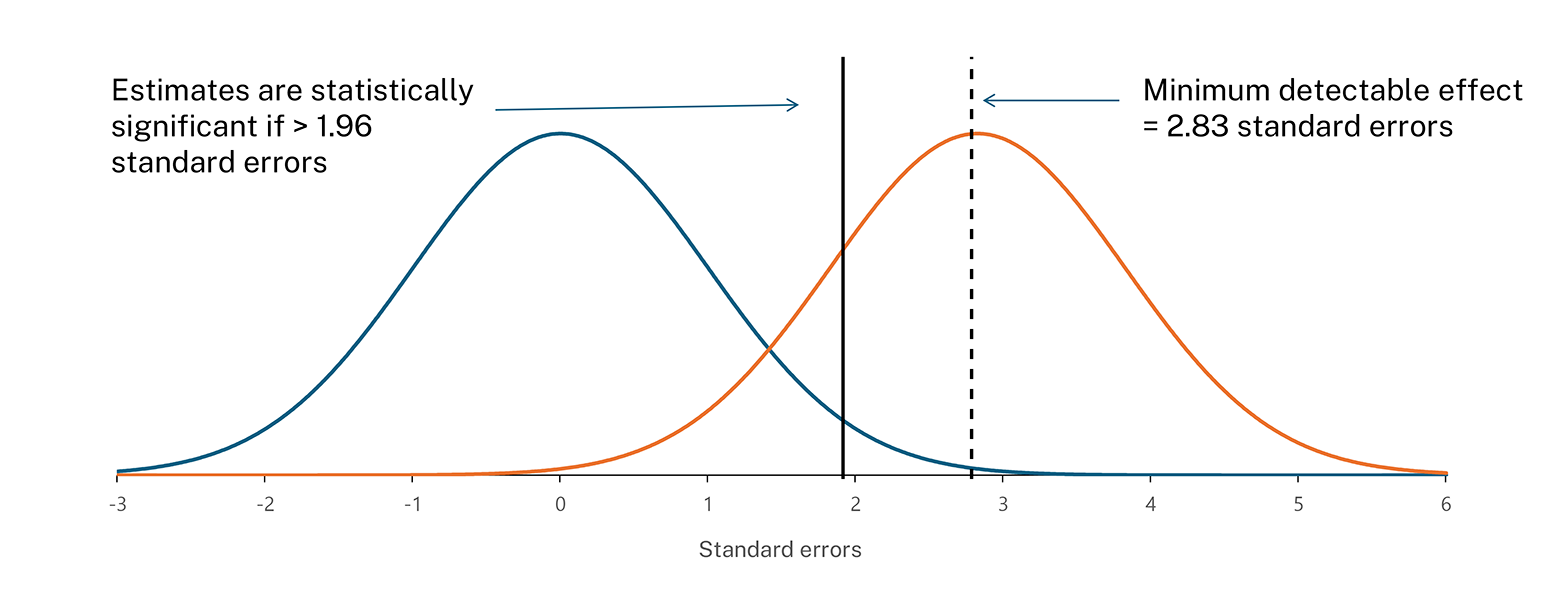
Key point: Estimates between 1.96 and 2.83 standard errors are statistically significant even though they are below the minimum detectable effect.
Finding the Minimum Detectable Effect
To understand how to find the minimum detectable effect, consider how it is defined:
The minimum detectable effect is the smallest true effect that will lead to a statistically significant estimated effect with probability equal to the study’s power.
In general, a study’s power is the probability of obtaining a statistically significant finding if the null hypothesis of zero effect is false (if the true effect is not zero). In calculating the minimum detectable effect, a study’s power is the probability of obtaining a statistically significant finding if the true effect is equal to the minimum detectable effect. A typical value for power is 80 percent, indicating a desire to design a study that has an 80 percent chance of producing a statistically significant finding if the true effect is equal to the minimum detectable effect.
If a study’s power is 80 percent and if estimates greater than 1.96 standard errors away from zero are different from 0 to a statistically significant degree, then the minimum detectable effect should be set so that 80 percent of estimates will be greater than 1.96 standard errors above 0 when the true effect equals the minimum detectable effect. In the figure, this set of criteria is represented by the orange bell curve, where 80 percent of the area lies to the right of 1.96 standard errors above 0. Using a 5 percent significance level with a two-tailed test, the bell curve that satisfies this criterion is centered at 2.83 standard errors above 0. That level is shown by the dashed vertical line. That is, the minimum detectable effect is 2.83 standard errors above 0.
The Relationship Between Statistically Significant Estimates and Minimum Detectable Effects
The information presented above indicates the following:
- Estimates greater than 1.96 standard errors from zero are statistically significant.
- The minimum detectable effect is 2.83 standard errors from zero.
Pulling these two pieces of information together shows that estimates below the minimum detectable effect—2.83 standard errors—will be statistically significant if they are greater than 1.96 standard errors. In other words, a study can produce statistically significant effect estimates even when its estimates are smaller than the study’s minimum detectable effect. As a rough rule of thumb, an effect estimate that is 70 percent as large as the minimum detectable effect will be statistically significant.
Implications for Researchers
Understanding the relationship between the minimum detectable effect and statistical significance has important implications for interpreting study results. When a study is being designed, the minimum detectable effect that is feasible to obtain is sometimes large, so it can be comforting to know the estimated effect can be smaller and still be statistically significant. If a study falls short of its enrollment target (which happens in many studies) the minimum detectable effect increases, and again it is important to remember that smaller estimates than the new minimum detectable effect will be statistically significant. This fact reflects the probabilistic nature of hypothesis testing: While the study was designed to detect effects as small as the minimum detectable effect with 80 percent probability, it can still detect smaller effects—just with lower probability.
When reporting results, it can be helpful to present both the minimum detectable effect (to show what the study was designed to detect) and the actual estimate with its standard error or confidence interval (to show what was found). This transparency helps readers understand both the study's capabilities and its findings.
[1] This assertion assumes inference is being made for a mean or difference in means, as would be the case for an impact analysis. The Central Limit Theorem shows that as the sample size gets larger, the distribution of an estimate of a mean gets closer to a normal distribution.
[2] The standard error is the standard deviation of the sampling distribution, indicating how much the estimated effect is expected to vary across repeated samples.
[3] This statement is true for a 5 percent significance level using a two-tailed test and a large enough sample. For a 10 percent significance level or a one-tailed test at the 5 percent significance level, the estimate would have to be more than 1.65 standard errors. For smaller samples, the critical value will be slightly larger, approaching 1.96 as sample size increases. For large samples (over 1,000 observations), 1.96 is close to exact.