Using Simulation to Analyze Interrupted Time Series


This post is one in a series highlighting MDRC’s methodological work. Contributors discuss the refinement and practical use of research methods being employed across our organization.
Hundreds of thousands of people in the United States are incarcerated in local jails as they wait for their criminal cases to be resolved. These people have not been convicted, but are incarcerated because they cannot afford to post bail.[1] Several jurisdictions, including Mecklenburg, North Carolina, have therefore instituted procedures meant to reduce the use of bail for “low-risk” defendants. Figure 1 shows what happened in Mecklenburg after those procedures were put in place. The line shows the proportion of arrests each month that resulted in bail or other restrictions on release before and after Mecklenburg’s reform. The dark gray indicates the post-policy era.[2]

The goal is to use these data to assess whether the policy affected the bail-setting rates, and if so, by how much. To do so, the trend before the policy change can be used to extrapolate what would have been seen had business continued as usual. If outcomes deviate from the projected trend, something probably changed the system to cause the departure.[3] The question is then how to do this extrapolation.
Simulating the Counterfactual Trend
One way to extrapolate how outcomes could rise and fall over time is to use simulation. A model is fit to all the pre-policy data, and then this model is used to simulate what would have happened had these trends continued. The model can, for example, incorporate information about how months close to each other are more similar than months further apart. The simulation approach used in this case is illustrated in Figures 2 and 3. Figure 2 shows 10 simulated extrapolations, each generated from a model fit to the pre-policy data. The team actually generated 10,000 such extrapolations, and summarized them by taking the middle 95 percent of the predictions for each time point. This middle range is shown as a green “prediction envelope” in Figure 3.
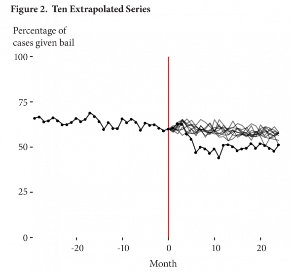

Overall the exercise shows evidence of a reduction in the use of bail: The actual bail rates are below the range of rates predicted by the pre-policy trends. It is also clear that outcomes for the first four months after the policy change are similar to the pre-policy trend; the departure is only significant beginning in Month 5, when actual bail levels off at a reduced rate of around 50 percent. Patterns such as these raise important issues of how to ascribe the change: Was this drop at Month 5 due to the policy shift, or due to some subsequent intervention that might not have been part of the policy? In Mecklenburg, there is some qualitative evidence that the county reinforced its policy change with additional training for court agents, which could have caused this delayed effect.
Note also that the pre-policy trend projects a steady decline in bail. For that reason, around two years after the policy was implemented, it is no longer possible to be sure it had an effect when compared with the extrapolation. The county may have reached those bail rates in the absence of the policy. But these further extrapolations make it important to consider the model carefully. One might ask, for example, whether the pre-policy trend could plausibly have continued for two more years in the absence of the intervention. The further out an extrapolation, the more important it is that the model be correctly specified, both statistically and as a representation of a dynamic and complex system.
Overall, there are three sources of uncertainty to attend to in such analyses as these, and only the first two are quantifiable: (1) parameter estimation error for the model, (2) natural variation due to month-to-month changes as captured by the model, and (3) model specification.
Conclusion
Simple modeling (linear regression with lagged outcomes and covariates) and a simulation framework can capture uncertainty for an interrupted time series design. The framework used in this study provides a picture of the evolution of a policy impact over time, rather than a single number summarizing overall impact. The above analyses and plots are all easily generated using an R package, simITS, that implements these methods.[4]
This simulation framework also allows for several extensions that can account for specific data concerns, improve the quality of the analysis, and improve the presentation and description of the results. The first such extension is smoothing: To make it easier to understand trends and detect deviations, smooth lines can be drawn through the more variable month-to-month sequences. These smoothed curves are arguably easier to read than the raw data. Smoothing also can increase power. See the full methods document for further details and examples.[5]
The simulation framework can also handle structural features of the data such as seasonality, where the outcome naturally rises and falls with the season (as total arrests tends to do). The Mecklenburg data did not extend far enough in the past for it to be possible to model seasonality, but in other, similar evaluation contexts this team approached, modeling seasonality proved essential for accurately extrapolating pre-policy trends.[6]
While the simulation approach is powerful, all an interrupted time series analysis can show — using this method or any other — is that the trend has changed in a surprising way. Why it did so, the statistics cannot answer. In the end, a researcher must turn to subject-matter knowledge and argument to defend the proposition that a change was caused by a policy shift.
[1]Zhen Zeng, Jail Inmates in 2016 (Washington, DC: Bureau of Justice Statistics, 2018).
[2]See a full evaluation of this initiative along with details of the intervention in Cindy Redcross and Brittany Henderson, with Luke Miratrix and Erin Valentine, Evaluation of Pretrial Justice System Reforms That Use the Public Safety Assessment: Effects in Mecklenburg County, North Carolina (New York: MDRC, 2019)
[3]A core assumption of this extrapolation is that the policy change had no effect until it was implemented. In other words, the data used to extrapolate must not be contaminated by possible effects of the policy. In some cases, to satisfy this assumption, one can move the point of the policy change earlier — for example, to when a policy was being planned rather than its official adoption date.
[4]This package, written by Luke Miratrix in collaboration with Brit Henderson and Chloe Anderson at MDRC, is available upon request. It will be published in the future on CRAN.
[5]Luke Miratrix, “Simulating for Uncertainty with Interrupted Time Series Designs,” unpublished paper (New York: MDRC, 2019).
[6]See, for example, Chloe Anderson Golub, Cindy Redcross, and Erin Jacobs Valentine, Evaluation of Pretrial Justice System Reforms That Use the Public Safety Assessment: Effects of New Jersey’s Criminal Justice Reform (New York: MDRC, 2019).